Histogram normalisation

Article by James Zjalic (Verden Forensics) and Foclar

Problem

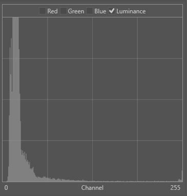
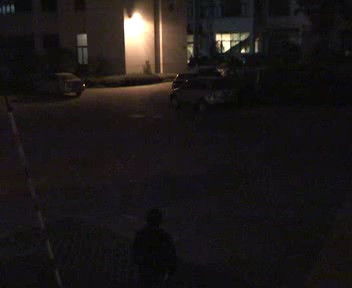
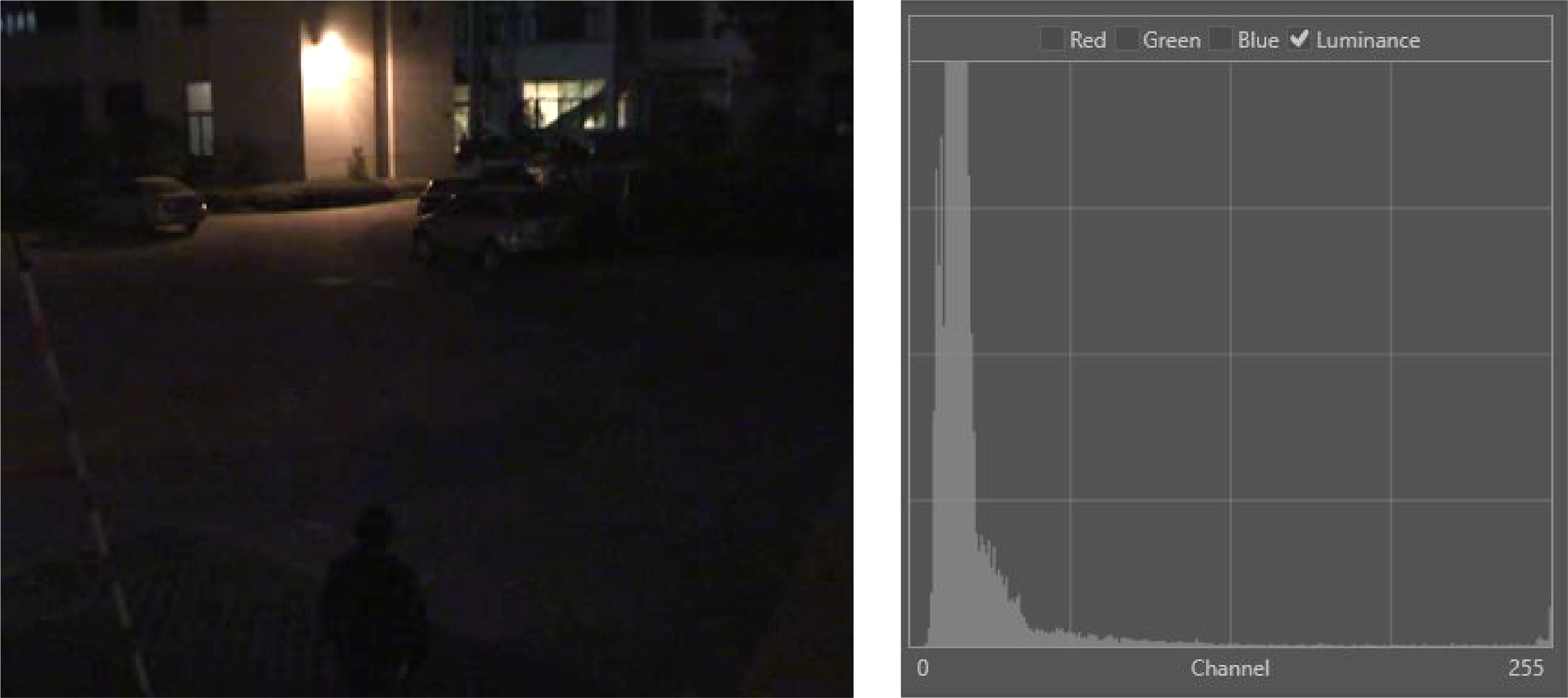
The majority of imagery used within forensics is captured under less than ideal conditions, be it a spontaneous capture using the camera on a mobile phone, or from a CCTV camera which is designed to cover a large area. As this imagery could contain evidence vital to a case, it is of the utmost importance that as much information as possible can be extracted from it, and as such, this means that in the vast majority of cases imagery could benefit from some form of enhancement. Although the type of processing required will be dependent on the specific quality issues and the instruction received, imagery with a skewed histogram distribution of pixel intensity values towards the extremes is an extremely common problem (Fig. 1). Often found within excessively light or dark captures (Fig. 2), this is a quality issue with a solution that provides the most value in terms of the increase in visual clarity it can deliver.

Cause

There are various reasons for a skewed distribution to the histogram of intensity values, but more often than not, it is due to the scene being too poorly or too intensely lit. A digital image capture of a dark environment will naturally contain fewer higher than lower pixel values, and in many instances, completely unoccupied bins in the upper regions of the histogram. This is often the case for CCTV captured during hours of darkness with little to no artificial lighting. Imagery captured during daylight hours (especially those on bright days) will contain a larger amount of higher intensity pixel values, and potentially unoccupied bins in the lower regions of the histogram. It may also be the case the capture conditions or device have resulted in unoccupied bins at both the upper and lower extremes.

Theory

When light hits a camera sensor, its magnitude is converted to an electrical representation, and as such, low-level light will be represented by lower voltages and vice versa. This continuous electrical information is then quantized to a discrete value within the range of 0 -255 (2⁸) for each pixel within each RGB layer. Light of lower intensity is, therefore quantized to lower values, whilst brighter light quantized to higher values [1]. When plotted on a histogram, the occurrence of each intensity value is visible, as is the distribution of such.

Solution

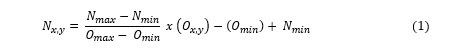
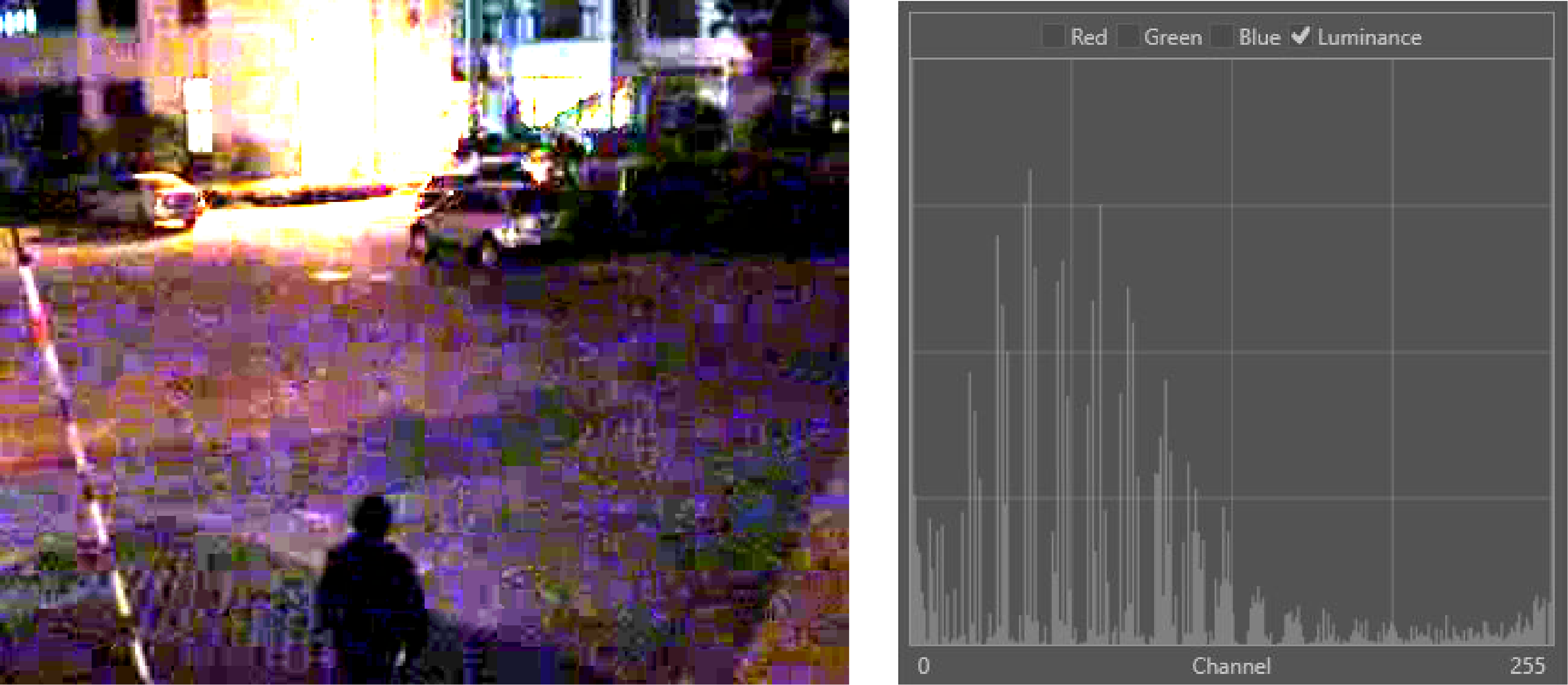
To correct this skewed distribution of intensity values, the optimal solution is to apply histogram normalisation, essentially stretching the limited range to cover the entire 256 values within the histogram. If the first bin occupied within the histogram of the original image is O_min, and the last O_max, the whole range can be stretched to between N_min (or 0) and N_max (or 255) using the following equation [2]:

A histogram adjustment maps (or proportionally scales) a range of intensities to the full range, thus amplifying the intensity differences between pixels. In doing this, the standard deviation of the luminance distribution is increased [3] and thus, the contrast of the imagery [4].

One of the problems which may limit the success of normalisation is the presence of both low intensity and high-intensity pixel values within an image with few bins occupied between these extremes. This is often the case for CCTV captured during hours of darkness in poorly lit environments containing vehicles with high-intensity headlights and reflective number plates. In cases like this, a decision must first be made as to the focus of the enhancement before the available options are considered. Only two options relating to normalisation will be covered in this article, but others will be looked at in future blogs. The first option is to crop to the region of interest, and the second is to subsample from a region of interest. In doing the former, the intensity values from the cropped out regions are removed, thus optimising the process. In doing the latter, the entire image is processed based on the pixel intensity values of a smaller region, and whilst this maintains the context, it can result in artefacts in other regions due to values being pushed above or beyond those available, and thus into under or overexposure. If there are multiple regions of interest required, multiple versions of the imagery, or cropped areas pertaining to each region would have to be created. Regardless of the method selected, the region from which the cropped image was obtained or subsampled must be documented, as must any unintended artefacts caused by the process [5].

Normalisation can be applied to each RGB channel in isolation, or the luminance (proportional to the intensity). Care must always be taken when applying it to individual channels to ensure the colour space balance is not disrupted, which may result in the misrepresentation of colours from with the capture environment.

There are a number of reasons to perform histogram normalisation, including the compression of the brightness range, equalisation of the camera response and to improve the contrast. The process of normalisation should always be one of, if not the first process performed during an enhancement in order to optimise all processes which follow [6]. It may also reduce the number of processes required as issues relating to brightness and contrast can be resolved.

Implementations

Foclar Impress provides a number of possible solutions for the previously described problems. It has a couple of predefined redistributions of the pixel values, including Stretch [7], Equalize [7] and Exposure [8].

The ‘Stretch’ filter is implemented according to formula (1). The ‘Equalize’ function aims to process the image in such a way that the resulting histogram is flat from 0-255, equalizing all level contributions. The ‘Exposure’ filter works in a similar way to the gain control on a hardware pre-amplifier, multiplying the incoming signal by a fixed factor.

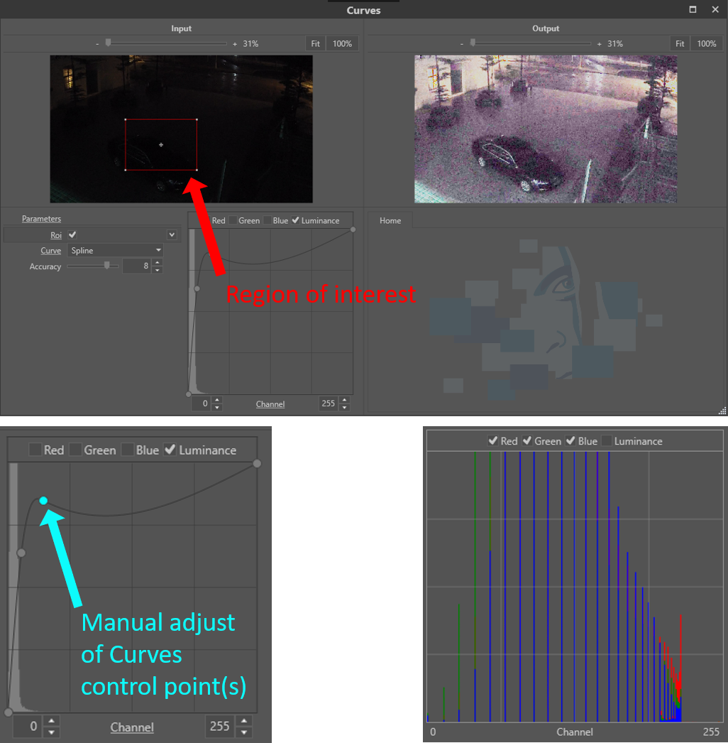
Impress also provides a manual method (entitled ‘Curves’) in which the user can change a curve manually to redistribute the pixel values [7], [9]. The optimal workflow is to adjust the curves in the detail window whilst simultaneously observing the histogram of the processed image to ensure an optimal distribution of the levels (Fig. 4). In some images, the intensity levels vary strongly over different regions. In these cases, the histogram of the region of interest can be used instead of the histogram of the total image.

Conclusion

A skewed histogram distribution is a common problem which can significantly reduce the clarity of evidence imagery. Redistributing the values to better fit the range of the histogram is a simple fix that may also reduce the number of other enhancement processes required. It can be achieved through a variety of techniques, and in order to know which is most applicable to the evidence imagery both an understanding of what an image histogram represents and the influence a particular method of redistribution is essential.

References

[1] Vlado Damjanovski, 2014. CCTV: From light to pixels, 3rd Edition. ed. Elsevier.

[2] Mark Nixon, Alberto Aguardo, 2002. Feature Extraction & Image Processing. Newnes.

[3] Mathworks, 2019. Image Processing in Matlab.

[4] Charles Poynton, 2007. Digital Video and HDTV: Algorithms and Interfaces. Elsevier.

[5] ENFSI, 2018. Best Practice Manual for Forensic Image and Video Enhancement.

[6] Spencer Ledesma, 2015. A Proposed Framework for image enhancement. University of Colorado, Denver.

[7] Alan C. Bovik, 2010. Handbook of Image and Video Processing. Academic Press.

[8] R. Szeliski, 2011. Computer Vision, Algorithms and Applications. Springer.

[9] M. Sonka, V. Hlavac, R. Boyle, 1999. Image Processing, Analysis and Machine Vision. Brooks/Cole Publishing Company.