Contrast adjustments

Article by James Zjalic (Verden Forensics) and Foclar

Problem

In order to obtain the optimal result for all imagery enhancement tasks, the examiner is required to achieve a delicate balance of feature emphasis whilst minimising artefacts. In no other process is this evidenced as much as when making contrast adjustments, where the overriding objective is to increase the ease at which images can be interpreted by making features of objects more distinguished. Poor contrast can potentially lead to features within the imagery being overlooked, or even misinterpreted due to the limited difference between pixel intensity values of different items within a scene. Although examples of low contrast can be found in all types of digital imagery, the lack of colour information within that from cameras which capture infrared video leads to a limited range of values to represent tones, and thus, the problem is more prevalent within this type of colour space.

In cases where the background and object, or feature within an object, are of extremely similar pixel intensity values (for example a black object held next to black trousers), no amount of contrast adjustment can improve the feature separation, as it is not possible to increase the difference between the pixels values representing each object to a degree which would be a) perceived by the human visual system (HVS) and b) not caused by compression.

Cause

Poor contrast within digital images is, as always, caused partly by the uncontrolled captured environment. Images which are excessively bright utilise fewer low intensity pixel values, and thus, the available dynamic range is reduced, which, in turn reduces the luminance difference between values. The same is true for imagery which is excessively dark, albeit in the lower regions when the intensity values are represented by a histogram. A further reason for low contrast is the poor sensitivity of CCD and CMOS sensors utilised by cameras leading to a lower narrow dynamic range than traditional film [1], [2].

A further factor which compounds the above is the high degree of compression of low frequency regions within a digital image or video, further reducing the contrast of that region.

Theory

Contrast can be thought of as the luminance difference between the brightest and darkest region of an image, where a small difference means the imagery has low contrast, and thus potentially poor feature separation, and a large difference means the imagery has a high contrast, and thus potentially good separation between features.

The human visual systems ability to differentiate between features is fundamentally informed by the JND, or Just Noticeable Difference. This is a measure of the change perceived by the HVS, determined by the amount of light necessary to add to a visual field such that it can be distinguished from the background [3].

Solution

Histogram Equalisation is a simple yet highly effective technique. Although it would make sense to apply this processing step within the capture device directly, therefore mitigating the need for post capture corrections, doing so can cause excessive contrast enhancement, resulting in a subsequent feature loss [1]. As such, contrast adjustments are performed in post-processing, typically through tone mapping techniques (function T) applied to the luminance values [4]. The method is a spatially invariant grey level transform [5], which can be defined by the following equation:

Y = T(x) (1)

As contrast adjustments increase the disparity between noise tonal values and the desired image signal, a by-product can be a visible increase in noise across an image. Contrast adjustments should always be performed prior to any sharpening functions to make it easier to identify areas for sharpening and the degree of sharpening to be applied. It should be noted that in low contrast images with large areas of colour, tone mapping will cause colour shifts, which can only be avoided by separate channel filtering.

Implementations

Foclar Impress provides various tone mapping functions (T). In this blog we only cover linear contrast enhancement, gamma correction and histogram equalisation. Examples of other possible mappings are logarithmic mapping, exposure correction, level inverse and histogram stretch.

For linear contrast [6-8], the mapping function T is implemented as a linear function (also covered in the previous blog article on brightness adjustment):

T(x) = C x + B (2)

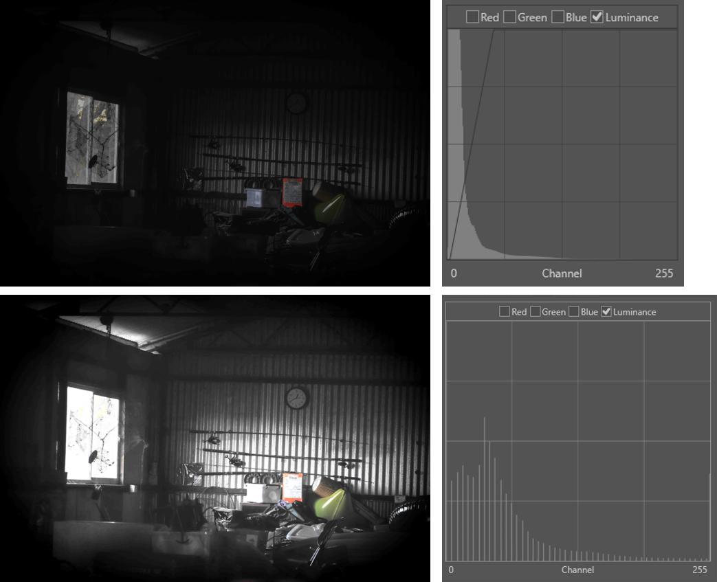
The filter has two parameters C (contrast) and B (brightness) which must be adjusted manually. The mapping function is shown in Fig. 1. The contrast determines the slope of the mapping function and the brightness the horizontal offset. Notice that the (grey) columns (tone levels present in the result image) in the resulting histogram are equally spaced, which is a result of the linear character of the mapping.

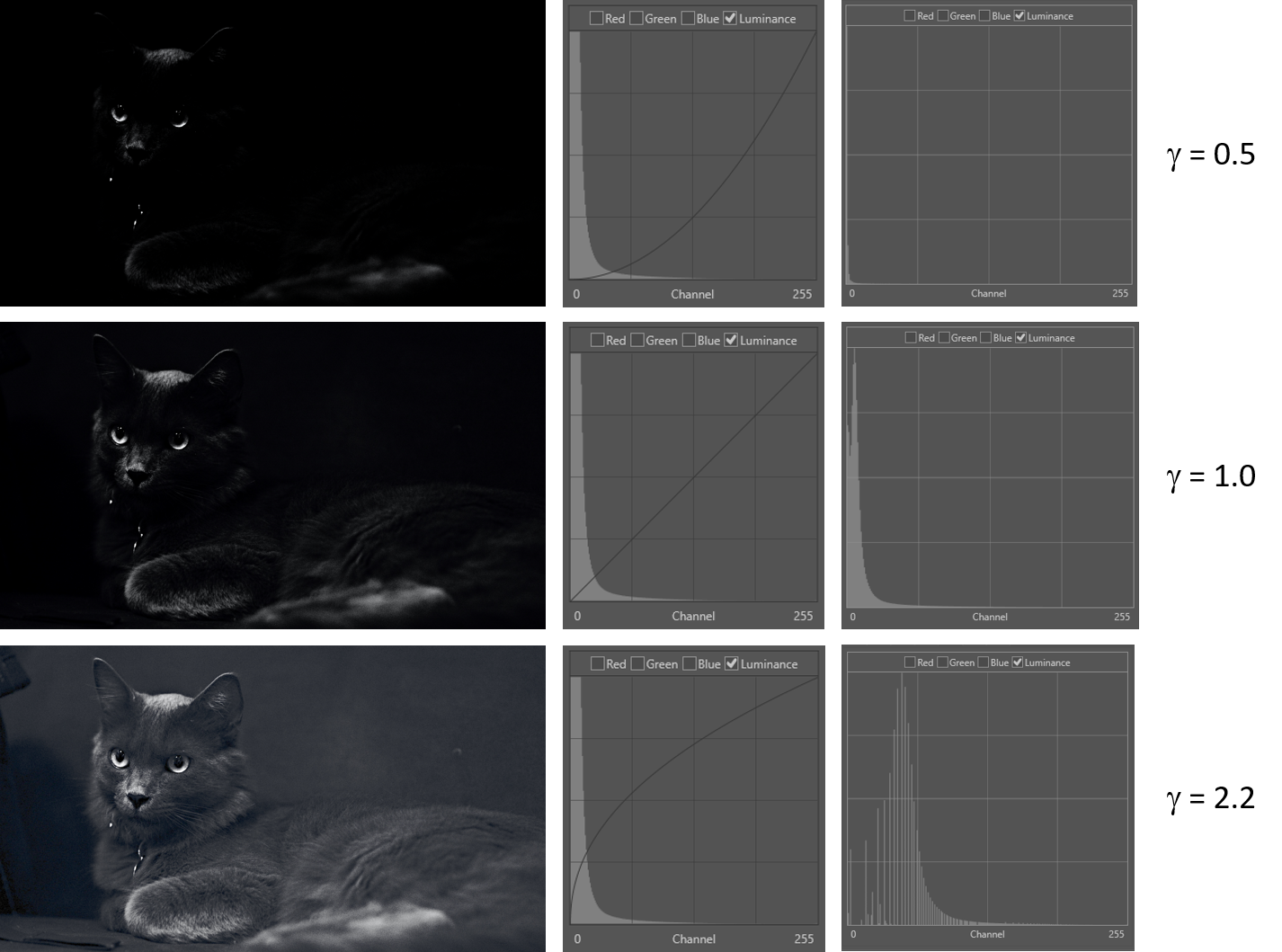
Gamma correction [9] originates from a correction function for the non-linear voltage-intensity response of CRT monitors (who still knows what these are?).

T(x) = x^{1 / g} (3)

This non-linear mapping function can also be used for non-linear contrast correction. The mapping is controlled by the parameter g (gamma). Figure 2 provides examples of the same image for different values of parameter gamma. The high tones have higher contrast for g=0.5, which can be useful in overexposed images. In case g=1.0, the mapping T becomes the identity mapping (T(x) = x). The gamma corrected image is equal to the original image. For g=2.2, (the better value for this image) the lower range shows larger distances between the tones when compared to the mid and high range (Figure 2, bottom row, histogram on the right).

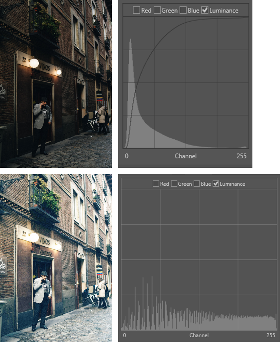
The last filter to be discussed in this article is the histogram equalisation filter [8]. The filter uses a tone mapping calculated from the accumulative histogram of the input image. The filter basically has no parameters and is different for each image. The mapping is designed to result in an approximately equal number of pixels of each tone in the filtered image. Figure 3 shows the application of the equalisation to a low contrast image. The histogram of the resulting image (bottom row, right histogram) is flat compared to the original histogram above, which also shows the mapping function used.

Conclusion

Adjustment of contrast in images is, like brightness, an important process to facilitate optimal interpretation of images and video frames, but it is vital that the introduction of artefacts and clipping is avoided to preserve as much information as possible. By simultaneously utilising a histogram and visual analysis to assess the imagery before selecting the appropriate linear or non-linear tone mapping function for a specific feature in a specific image will ensure optimal results.

References

[1] C.-C. Chiu and C.-C. Ting, “Contrast Enhancement Algorithm Based on Gap Adjustment for Histogram Equalization,” Sensors, vol. 16, no. 6, p. 936, Jun. 2016, doi: 10.3390/s16060936.

[2] John C. Russ, Forensic Uses of Digital Imaging. CRC Press, 2001.

[3] G. Buchsbaum, “An Analytical Derivation of Visual Nonlinearity,” IEEE Trans. Biomed. Eng., vol. BME-27, no. 5, pp. 237–242, May 1980, doi: 10.1109/TBME.1980.326628.

[4] M. Bressan, C. R. Dance, H. Poirier, and D. Arregui, “Local contrast enhancement,” San Jose, CA, USA, Jan. 2007, p. 64930Y, doi: 10.1117/12.724721.

[5] M. Grundland and N. A. Dodgson, “Automatic Contrast Enhancement by Histogram Warping,” in Computer Vision and Graphics, vol. 32, K. Wojciechowski, B. Smolka, H. Palus, R. S. Kozera, W. Skarbek, and L. Noakes, Eds. Dordrecht: Springer Netherlands, 2006, pp. 293–300.

[6] Sonka M. Hlavac V. Boyle R. (1999) Image Processing, Analysis and Machine Vision, p10, 33 Brooks/Cole Publishing Company.

[7] R. Szeliski (2011) Computer Vision, Algorithms and Applications, p91 Springer.

[8] Alan C. Bovik (2010) Handbook of Image and Video Processing, p27 Academic Press.

[9] R. Szeliski (2011) Computer Vision, Algorithms and Applications, p77 Springer.