Blur

Article by James Zjalic (Verden Forensics) and Foclar

Problem

Blur is a historical problem for which solutions have been studied over a number of decades. Its root cause is the inability of an imaging system to focus on objects on an image plane at the same time, or relative motion between a camera lens and an object during exposure. The uncontrolled and varying conditions of forensic imagery can result in both of these causes being realised, and thus it is extremely common for both images and video to require some form of de-blurring within the sequence of enhancement operators applied to recover high-frequency information, and thus detail.

Cause

The issue itself is caused by the convolution of an original image with a point spread function (PSF; the output of a system in relation to a point source input). Examples of types of blur within forensics include:

• Linear Motion Blur.
  The result of relative motion between a camera viewpoint and the source during exposure time. It can be worse in low light conditions where longer exposure times are required.
• Rotational Motion Blur.
  The result of the relative motion when a camera approaches an object at high speed.
• Defocus.
  Objects near the camera are sharp, whereas those in the distance are blurred.
• Radial blur.
  A type of defocus caused by the inherent defect of an imaging system such as a single lens, characterised by an image which is sharp at the centre and blurred as the distance from the central plane increases

(Zhang and Ueda, 2011)

In a worst-case scenario, the difficulties are compounded when a number of the above exist, for example where the camera is in motion, and the subjects appear at different distances from the camera lens moving in different directions. When it is considered that other issues may also exist, including those related to noise and colours, it is likely that the quality of an image will be limited by such.

Theory

When an image is captured, the lens does not focus a single point to a corresponding point on the sensor, and thus the colour information pertaining to an object is diffused from a central region. The magnitude and direction of this spread can be considered to be the point spread function.

Blur is caused by the convolution (X) of the latent (or true image) with the point spread function, as below, where B represents the blurred image, I the latent image, and n the noise.

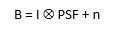
(1) 

(Pan et al., 2019)

Solution

In cases where the PSF is known, such as the Hubble telescope, it is possible to de-convolve the PSF from the provided image to obtain the original image. In most practical applications, including forensics, the PSF is not known as the content of the capture cannot be predicted. The presence and correction of blur is therefore known as a blind de-convolution process, in which a sequential approach is utilised by first estimating the PSF and then de-convolving the blurred image. The estimation process is generally iterative, in which estimation is made followed by adjustments. The most common method is to model the PSF is a shift-invariant kernel (Bar et al., 2006). A key limitation as it applies to forensics is that this model assumes that the degree and direction of blur is uniform across the image, which is not necessarily the case (again, consider two subjects running in opposing directions). The selected PSF will therefore either be a compromise and thus the blur will not be as reduced as much as it could be, or will reduce the blur pertaining to one element whilst likely increasing the blur relating to the other (Hu and Yang, 2015; Russ, 2001).

The process of reducing blur is known as de-blur, and considerations for its position in the order of operations must be made. As sharpening increases the contrast between high-frequency regions, and blur reduces high-frequency information, the result of sharpening a blurred image would be sub-optimal. It must also be considered that colours within a blurred image are diffused throughout due to the convolution with the PSF, and so colour adjustments cannot be accurately applied. It is therefore recommended that any de-blur process is performed prior to these operations (Ledesma, 2015).

Implementations

In Impress a number of different types of de-blur filters are available [7], [8], including for linear motion, general misfocus, and custom de-blur. The operator has to select the blue filter, which is most appropriate for the image of interest. The algorithm used for all de-blur filters is the Wiener filter, with differences between the above mentioned de-blur filters being caused by the shape of the PSF used by the Wiener filter. To be able to explain the way is filter works, first, the power spectrum has to be introduced.

Power spectrum

The power spectrum is an alternative way to characterise a signal. For example, a sinusoid shaped audio waveform can be described as a single frequency (Figure 1).

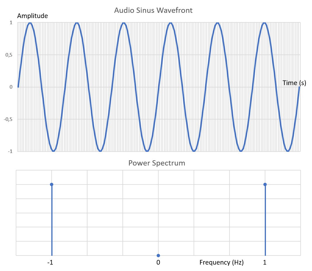
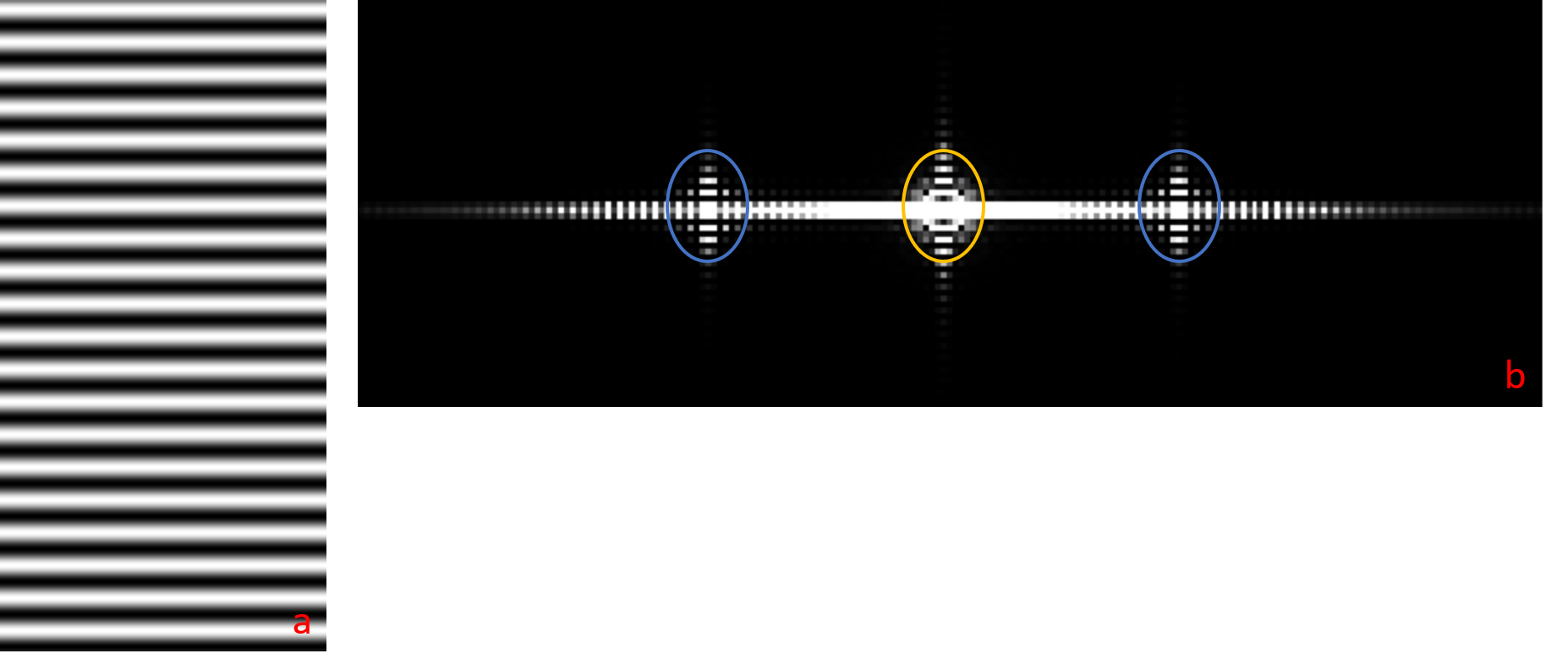
A one-dimensional time signal is decomposed in one or more frequencies (in this case a single frequency), displayed in the one-dimensional power spectrum. Similarly, an image with two spatial coordinates in pixels can be decomposed into a two-dimensional power spectrum. This is shown in Figure 2, where an image with a sine wave results in a power spectrum with two main frequencies inside the blue ellipses. The origin is indicated by the yellow ellipse (frequency value zero), which corresponds to the average brightness level in the image. The outer areas of the power spectrum correspond to the high frequencies in the image. The high frequencies represent both noise signal and the fine details of the image (sharp contours). Notice that the axis in the power spectrum is rotated over 90 degrees relative to the direct space image coordinates. A natural image can be considered to be build up by many sine waves of different magnitudes (amplitudes), frequencies, directions and starting points (phase). The power spectrum of a natural image is, therefore, more complex, see for example Figure 3.

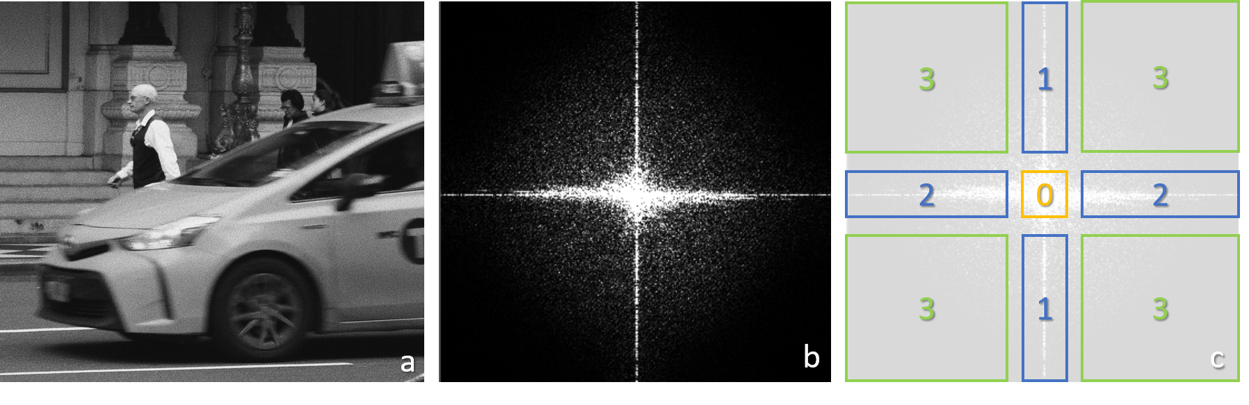
The mathematical transformation to calculate the audio power spectrum going from time (seconds) to frequencies (Hz) is the Fourier transform. Similarly, the two-dimensional Fourier transform is used to calculate the power spectrum of an image, going from direct space pixels (Figure 2a, 3a) to frequency pixels (Figure 2b, 3b).

Fourier transform

This Wiener filter uses the Fourier transform (and its inverse transform) as a mathematical tool to estimate the latent (sharp) image I from the blurry image B. The trick is to transform the equation (1) to its Fourier equivalent:

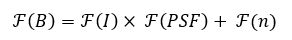
(2)

This way, the complex convolution operation (Ä) for direct space pixels changes into a simple frequency pixel by pixel multiplication (x). This equation can be solved for I if PSF and n are known, giving:

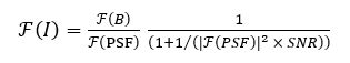
(3)

with SNR being the signal-to-noise ratio of the image.

The final step is to inverse Fourier transform the result (3) to recover the latent image:

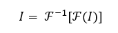
(4)

Linear motion deblur

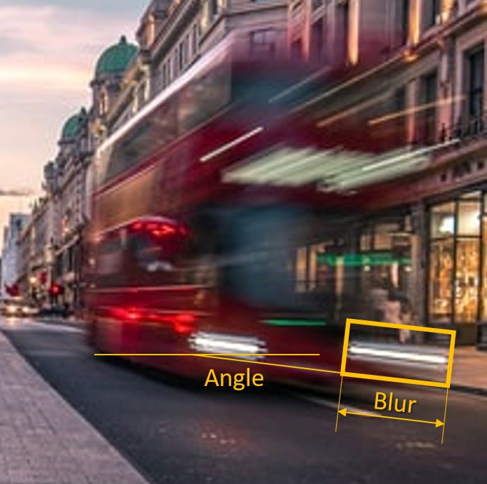
During the shutter time of the recording of a single frame or still image, the camera or object(s) of interest or both can move. If the motion is fast relative to the duration of the shutter time, this results in so-called blur streaks. To compensate for the effect the Blur parameter should have a value which corresponds to the length of the blur streak. The Angle parameter should correspond to the angle between the streak and the horizontal axis. Both parameters control the shape and extent of the PSF function of formula (1).

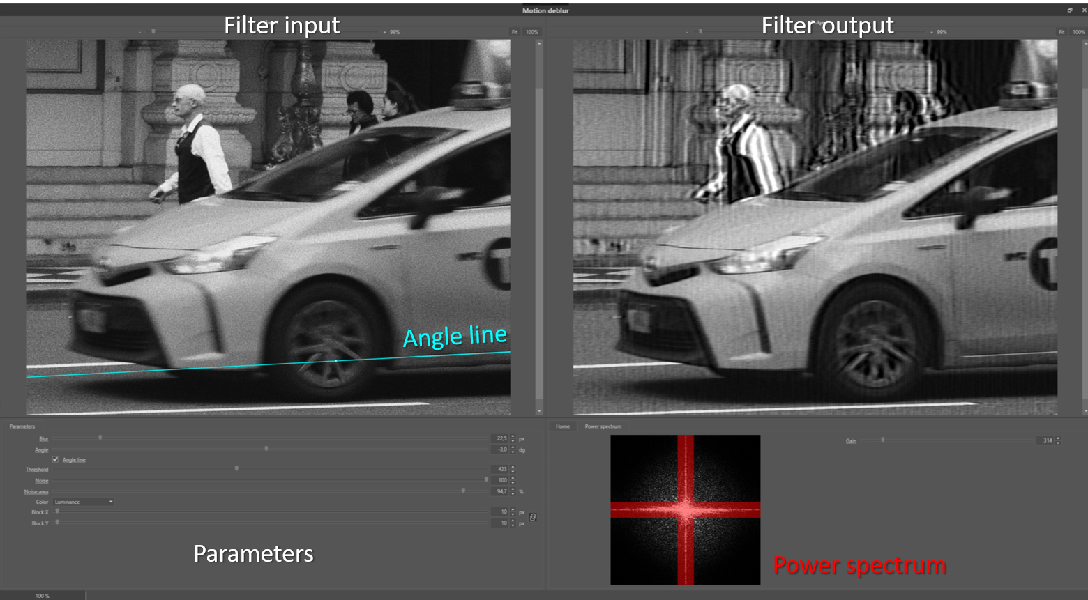
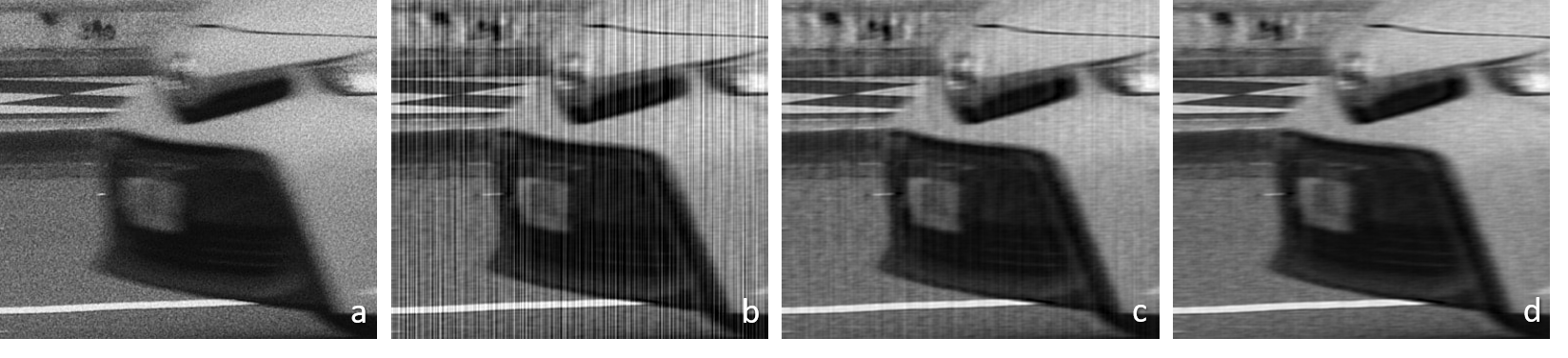
In real-life cases, the blur streaks (Figure 4) might be less obvious to find, see, for example Figure 5 and 6. The noise signal is estimated from the outer areas of the power spectrum. In Figure 7 this corresponds to the non-red areas. With the Noise Area parameter, which acts as a cut off between signal and noise frequencies, these areas can be adjusted. If the image contains many high-frequency features, decreasing the parameter value will help to preserve these. The Noise parameter allows the operator to tune the strength of the noise compensation of the filter. In Figure 8, the de-blur result on the front end of the taxi is displayed for different values of the so-called threshold parameter. This parameter suppresses wave-like distortions in the result images. If the parameter is chosen too large, the de-blur compensation is not so effective anymore. The color parameter enables the de-blur on the luminance or individual colour channels.

Misfocus

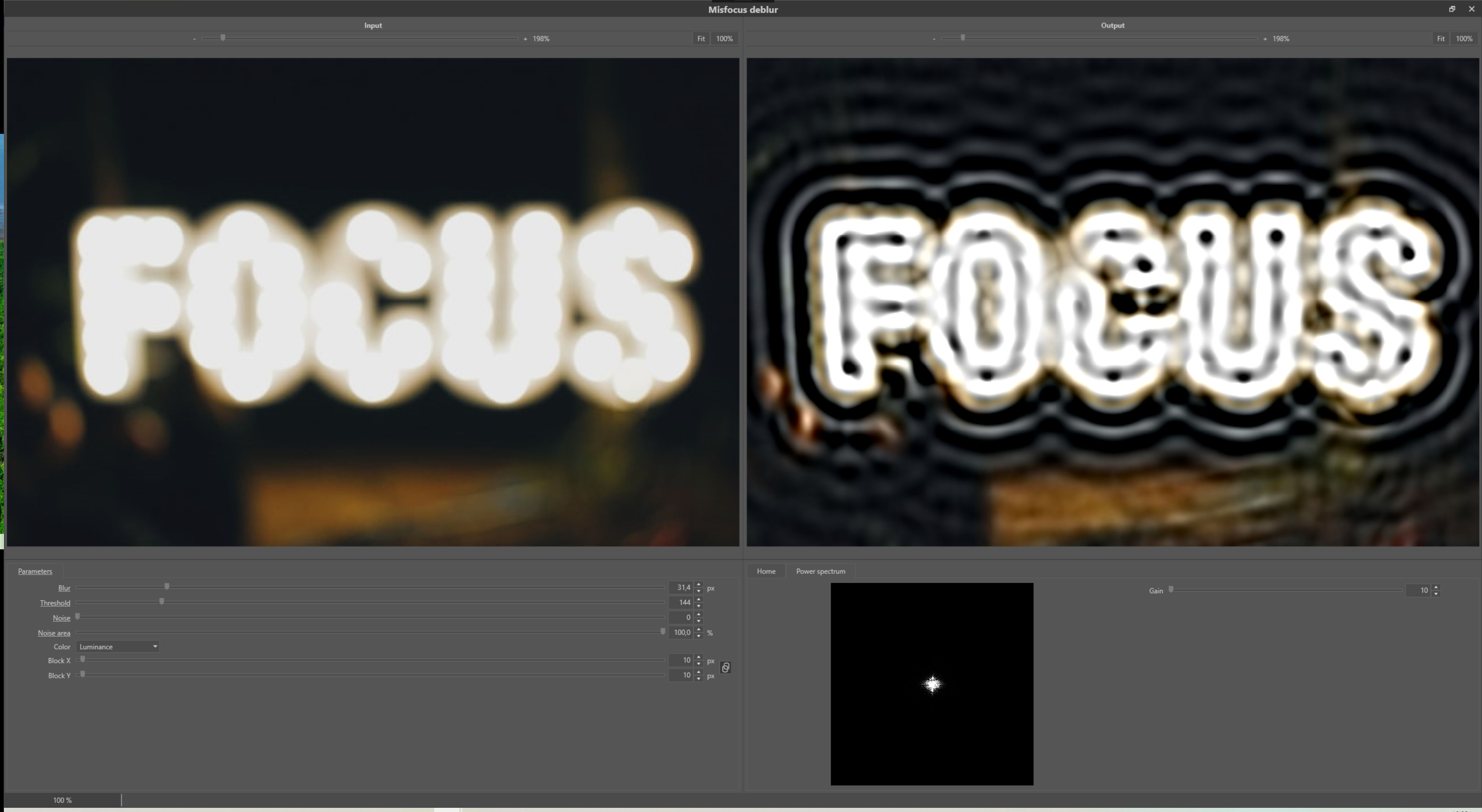
Examples of misfocus are shown in Figure 9 and 10. The blur effect has the shape of circles. The misfocus de-blur or defocus filter should have a Blur parameter value corresponding to the radius of the blur circles.

General de-blur

The general or thermal de-blur filter uses a Gaussian PSF function (formula (1)). The Gaussian function can, for example, be used to model atmospheric turbulence accurately. This filter is also very useful for post-processing of super-resolution images, and as a general sharpen filter in cases where the blur source in the image is the result of many blur sources. The parameter settings are similar to the misfocus de-blur filter.

Custom de-blur

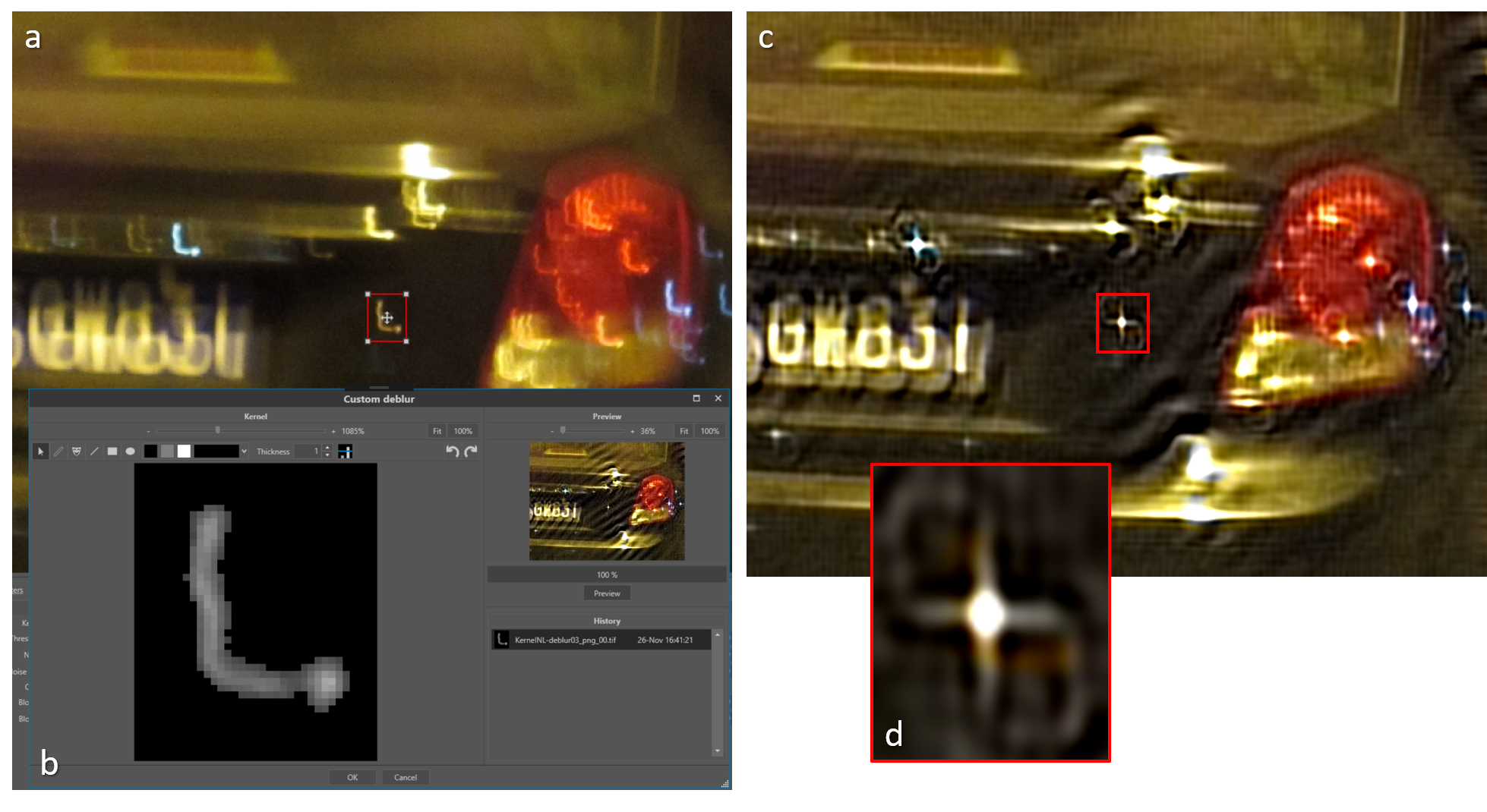
In case the blur effect in an image is caused by non-linear motion or a complex composition of multiple blur types, one can apply the so-called custom de-blur filter. In Figure 11 an example is shown of a non-linear accelerated motion. The motion blur, in this case, is very complex, and so could not be modelled by a curved line, since the motion was accelerated, resulting in intensity variations along the curve. If the blur kernel feature can be isolated, it can be used to compensate for the complex blur pattern it represents. Ideally, the blur kernel is in the filtered image changed into a single dot. Therefore, if one knows that some blurry feature in an image should originate from a point-like shape, one can use this blurry feature for extraction of the blur kernel using the custom de-blur filter. The above extraction procedure is independent of the complexity of the blur pattern in the image. The only condition is that it should be possible to separate the blur feature from the background. To further facilitate this process, extra ‘drawing’ options (Figure 11 b) are available to retouch the extracted blur kernel. The hash of the extracted kernel image is included in the processing log to guarantee reproducibility.

Conclusion

Although the requirement for assumptions to be made in relation to the unknown point spread function prior to de-convolution can cause limitations in the results of de-blurring, when a good estimate is achieved the results can be highly effective.

References

[1] Bar, L., Kiryati, N., Sochen, N., 2006. Image Deblurring in the Presence of Impulsive Noise. Int. J. Comput. Vis. 70, 279–298. https://doi.org/10.1007/s11263...

[2] Hu, Z., Yang, M.-H., 2015. Learning Good Regions to Deblur Images. Int. J. Comput. Vis. 115, 345–362. https://doi.org/10.1007/s11263...

[3] Ledesma, S., 2015. A Proposed Framework for image enhancement. University of Colorado, Denver.

[4] Pan, J., Ren, W., Hu, Z., Yang, M.-H., 2019. Learning to Deblur Images with Exemplars. IEEE Trans. Pattern Anal. Mach. Intell. 41, 1412–1425. https://doi.org/10.1109/TPAMI....

[5] Russ, J.C., 2001. Forensic Uses of Digital Imaging. CRC Press.

[6] Zhang, Y., Ueda, T., 2011. Deblur of radially variant blurred image for single lens system. IEEE Trans. Electr. Electron. Eng.

[7] Sonka, M., Hlavac, V., Boyle, R., 1999. Image Processing, Analysis and Machine Vision, p106. Brooks /Cole Publishing Company.

[8] Bovik, A.C., 2010, Handbook of Image and Video Processing, p173. Academic Press.